04. Performance Profiling

We can profile the performance with a 3D FDTD simulation:

Imports

import matplotlib.pyplot as plt
from line_profiler import LineProfiler

import fdtd
import fdtd.backend as bd

Set Backend

Let’s profile the impact of the backend. These are the possible backends:

• numpy (defaults to float64 arrays)

• torch (defaults to float64 tensors)

• torch.float32

• torch.float64

• torch.cuda (defaults to float64 tensors)

• torch.cuda.float32

• torch.cuda.float64

fdtd.set_backend("numpy")

In general, the numpy backend is preferred for standard CPU calculations with "float64" precision as it is slightly faster than torch backend on CPU. However, a significant performance improvement can be obtained by choosing torch.cuda on large enough grids.

Note that, in FDTD, float64 precision is generally preferred over float32 to ensure numerical stability and prevent numerical dispersion. If this is of no concern to you, you can opt for float32 precision, which especially on a GPU might yield a significant performance boost.

Constants

WAVELENGTH = 1550e-9
SPEED_LIGHT: float = 299_792_458.0  # [m/s] speed of light

Setup Simulation

create FDTD Grid

N = 100

grid = fdtd.Grid(
    (N, N, N),
    grid_spacing=0.05 * WAVELENGTH,
    permittivity=1.0,
    permeability=1.0,
)

add boundaries

# x boundaries
grid[0:10, :, :] = fdtd.PML(name="pml_xlow")
grid[-10:, :, :] = fdtd.PML(name="pml_xhigh")

# y boundaries
grid[:, 0:10, :] = fdtd.PML(name="pml_ylow")
grid[:, -10:, :] = fdtd.PML(name="pml_yhigh")

# z boundaries
grid[:, :, 0:10] = fdtd.PML(name="pml_zlow")
grid[:, :, -10:] = fdtd.PML(name="pml_zhigh")

add sources

grid[10+N//10:10+N//10, :, :] = fdtd.PlaneSource(
    period=WAVELENGTH / SPEED_LIGHT, name="source"
)

add objects

grid[10+N//5:4*N//5-10, 10+N//5:4*N//5-10, 10+N//5:4*N//5-10] = fdtd.Object(permittivity=2.5, name="center_object")

grid summary

print(grid)

Grid(shape=(100,100,100), grid_spacing=7.75e-08, courant_number=0.57)

sources:
    PlaneSource(period=35, amplitude=1.0, phase_shift=0.0, name='source', polarization='z')
        @ x=[20, ... , 21], y=[0, ... , 100], z=[0, ... , 100]

boundaries:
    PML(name='pml_xlow')
        @ x=0:10, y=:, z=:
    PML(name='pml_xhigh')
        @ x=-10:, y=:, z=:
    PML(name='pml_ylow')
        @ x=:, y=0:10, z=:
    PML(name='pml_yhigh')
        @ x=:, y=-10:, z=:
    PML(name='pml_zlow')
        @ x=:, y=:, z=0:10
    PML(name='pml_zhigh')
        @ x=:, y=:, z=-10:

objects:
    Object(name='center_object')
        @ x=30:70, y=30:70, z=30:70

Setup LineProfiler

create and enable profiler

profiler = LineProfiler()
profiler.add_function(grid.update_E)
profiler.enable()

Run Simulation

run simulation

grid.run(50, progress_bar=True)

100%|██████████| 50/50 [00:13<00:00,  3.73it/s]

Profiler Results

print profiler summary

profiler.print_stats()

Timer unit: 1e-09 s

Total time: 6.6444 s
File: /home/docs/checkouts/readthedocs.org/user_builds/fdtd/checkouts/latest/docs/examples/fdtd/grid.py
Function: update_E at line 275

Line #      Hits         Time  Per Hit   % Time  Line Contents
==============================================================
   275                                               def update_E(self):
   276                                                   """update the electric field by using the curl of the magnetic field"""
   277
   278                                                   # update boundaries: step 1
   279       300     451320.0   1504.4      0.0          for boundary in self.boundaries:
   280       300 2487669484.0 8292231.6     37.4              boundary.update_phi_E()
   281
   282        50 2859277211.0 57185544.2     43.0          curl = curl_H(self.H)
   283        50  746051675.0 14921033.5     11.2          self.E += self.courant_number * self.inverse_permittivity * curl
   284
   285                                                   # update objects
   286        50     194228.0   3884.6      0.0          for obj in self.objects:
   287        50   72522680.0 1450453.6      1.1              obj.update_E(curl)
   288
   289                                                   # update boundaries: step 2
   290       300     340996.0   1136.7      0.0          for boundary in self.boundaries:
   291       300  474581196.0 1581937.3      7.1              boundary.update_E()
   292
   293                                                   # add sources to grid:
   294        50      93652.0   1873.0      0.0          for src in self.sources:
   295        50    3177339.0  63546.8      0.0              src.update_E()
   296
   297                                                   # detect electric field
   298        50      43737.0    874.7      0.0          for det in self.detectors:
   299                                                       det.detect_E()

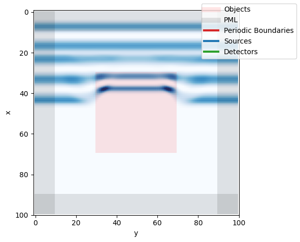
Visualization

plt.figure()
grid.visualize(z=N//2)