Python 3D FDTD Simulator

A 3D electromagnetic FDTD simulator written in Python. The FDTD simulator has an optional PyTorch backend, enabling FDTD simulations on a GPU.

Docs

• Examples
  • 00. Quick Start
  • 01. Basic Example
  • 02. Absorbing Object
  • 03. Objects of arbitrary shape
  • 04. Performance Profiling
  • 05. Lenses and analysing lensing actions
  • 06. GRIN medium and analysing refraction
• fdtd package
  • backend module
  • boundaries module
  • detectors module
  • grid module
  • objects module
  • sources module

Installation

The fdtd-library can be installed with pip:

pip install fdtd

Dependencies

• python 3.6+

• numpy

• matplotlib

• tqdm

• pytorch (optional)

Quick intro

The fdtd library is simply imported as follows:

import fdtd

Setting the backend

fdtd.backend

The fdtd library allows to choose a backend. The "numpy" backend is the default one, but there are also several additional PyTorch backends:

• numpy (defaults to float64 arrays)

• torch (defaults to float64 tensors)

• torch.float32

• torch.float64

• torch.cuda (defaults to float64 tensors)

• torch.cuda.float32

• torch.cuda.float64

For example, this is how to choose the torch backend:

fdtd.set_backend("torch")

In general, the numpy backend is preferred for standard CPU calculations with float64 precision. In general, float64 precision is always preferred over float32 for FDTD simulations, however, float32 might give a significant performance boost.

The cuda backends are only available for computers with a GPU.

The FDTD-grid

fdtd.grid

The FDTD grid defines the simulation region.

# signature
fdtd.Grid(
    shape: Tuple[Number, Number, Number],
    grid_spacing: float = 155e-9,
    permittivity: float = 1.0,
    permeability: float = 1.0,
    courant_number: float = None,
)

A grid is defined by its shape, which is just a 3D tuple of Number-types (integers or floats). If the shape is given in floats, it denotes the width, height and length of the grid in meters. If the shape is given in integers, it denotes the width, height and length of the grid in terms of the grid_spacing. Internally, these numbers will be translated to three integers: grid.Nx, grid.Ny and grid.Nz.

A grid_spacing can be given. For stability reasons, it is recommended to choose a grid spacing that is at least 10 times smaller than the _smallest_ wavelength in the grid. This means that for a grid containing a source with wavelength 1550nm and a material with refractive index of 3.1, the recommended minimum grid_spacing turns out to be 50pm

For the permittivity and permeability floats or arrays with the following shapes

• (grid.Nx, grid.Ny, grid.Nz)

• or (grid.Nx, grid.Ny, grid.Nz, 1)

• or (grid.Nx, grid.Ny, grid.Nz, 3)

are expected. In the last case, the shape implies the possibility for different permittivity for each of the major axes (so-called _uniaxial_ or _biaxial_ materials). Internally, these variables will be converted (for performance reasons) to their inverses grid.inverse_permittivity array and a grid.inverse_permeability array of shape (grid.Nx, grid.Ny, grid.Nz, 3). It is possible to change those arrays after making the grid.

Finally, the courant_number of the grid determines the relation between the time_step of the simulation and the grid_spacing of the grid. If not given, it is chosen to be the maximum number allowed by the Courant-Friedrichs-Lewy Condition: 1 for 1D simulations, 1/√2 for 2D simulations and 1/√3 for 3D simulations (the dimensionality will be derived by the shape of the grid). For stability reasons, it is recommended not to change this value.

grid = fdtd.Grid(
    shape = (25e-6, 15e-6, 1), # 25um x 15um x 1 (grid_spacing) --> 2D FDTD
)
print(grid)

Grid(shape=(161,97,1), grid_spacing=1.55e-07, courant_number=0.70)

Objects

fdtd.objects

An other option to locally change the permittivity or permeability in the grid is to add an Object to the grid.

# signature
fdtd.Object(
    permittivity: Tensorlike,
    name: str = None
)

An object defines a part of the grid with modified update equations, allowing to introduce for example absorbing materials or biaxial materials for which mixing between the axes are present through Pockels coefficients or many more. In this case we’ll make an object with a different permittivity than the grid it is in.

Just like for the grid, the Object expects a permittivity to be a floats or an array of the following possible shapes

• (obj.Nx, obj.Ny, obj.Nz)

• or (obj.Nx, obj.Ny, obj.Nz, 1)

• or (obj.Nx, obj.Ny, obj.Nz, 3)

Note that the values obj.Nx, obj.Ny and obj.Nz are not given to the object constructor. They are in stead derived from its placing in the grid:

grid[11:32, 30:84, 0] = fdtd.Object(permittivity=1.7**2, name="object")

Several things happen here. First of all, the object is given the space [11:32, 30:84, 0] in the grid. Because it is given this space, the object’s Nx, Ny and Nz are automatically set. Furthermore, by supplying a name to the object, this name will become available in the grid:

print(grid.object)

Object(name='object')
    @ x=11:32, y=30:84, z=0:1

A second object can be added to the grid:

grid[13e-6:18e-6, 5e-6:8e-6, 0] = fdtd.Object(permittivity=1.5**2)

Here, a slice with floating point numbers was chosen. These floats will be replaced by integer Nx, Ny and Nz during the registration of the object. Since the object did not receive a name, the object won’t be available as an attribute of the grid. However, it is still available via the grid.objects list:

print(grid.objects)

[Object(name='object'), Object(name=None)]

This list stores all objects (i.e. of type fdtd.Object) in the order that they were added to the grid.

Sources

fdtd.sources

Similarly as to adding an object to the grid, an fdtd.LineSource can also be added:

# signature
fdtd.LineSource(
    period: Number = 15, # timesteps or seconds
    amplitude: float = 1.0,
    phase_shift: float = 0.0,
    name: str = None,
)

And also just like an fdtd.Object, an fdtd.LineSource size is defined by its placement on the grid:

grid[7.5e-6:8.0e-6, 11.8e-6:13.0e-6, 0] = fdtd.LineSource(
    period = 1550e-9 / (3e8), name="source"
)

However, it is important to note that in this case a LineSource is added to the grid, i.e. the source spans the diagonal of the cube defined by the slices. Internally, these slices will be converted into lists to ensure this behavior:

print(grid.source)

LineSource(period=14, amplitude=1.0, phase_shift=0.0, name='source')
    @ x=[48, ... , 51], y=[76, ... , 83], z=[0, ... , 0]

Note that one could also have supplied lists to index the grid in the first place. This feature could be useful to create a LineSource of arbitrary shape.

Detectors

fdtd.detectors

# signature
fdtd.LineDetector(
    name=None
)

Adding a detector to the grid works the same as adding a source

grid[12e-6, :, 0] = fdtd.LineDetector(name="detector")
print(grid.detector)

LineDetector(name='detector')
    @ x=[77, ... , 77], y=[0, ... , 96], z=[0, ... , 0]

Boundaries

fdtd.boundaries

# signature
fdtd.PML(
    a: float = 1e-8, # stability factor
    name: str = None
)

Although, having an object, source and detector to simulate is in principle enough to perform an FDTD simulation, One also needs to define a grid boundary to prevent the fields to be reflected. One of those boundaries that can be added to the grid is a Perfectly Matched Layer: or PML. These are basically absorbing boundaries.

# x boundaries
grid[0:10, :, :] = fdtd.PML(name="pml_xlow")
grid[-10:, :, :] = fdtd.PML(name="pml_xhigh")

# y boundaries
grid[:, 0:10, :] = fdtd.PML(name="pml_ylow")
grid[:, -10:, :] = fdtd.PML(name="pml_yhigh")

Grid Summary

A simple summary of the grid can be shown by printing out the grid:

print(grid)

Grid(shape=(161,97,1), grid_spacing=1.55e-07, courant_number=0.70)

sources:
    LineSource(period=14, amplitude=1.0, phase_shift=0.0, name='source')
        @ x=[48, ... , 51], y=[76, ... , 83], z=[0, ... , 0]

detectors:
    LineDetector(name='detector')
        @ x=[77, ... , 77], y=[0, ... , 96], z=[0, ... , 0]

boundaries:
    PML(name='pml_xlow')
        @ x=0:10, y=:, z=:
    PML(name='pml_xhigh')
        @ x=-10:, y=:, z=:
    PML(name='pml_ylow')
        @ x=:, y=0:10, z=:
    PML(name='pml_yhigh')
        @ x=:, y=-10:, z=:

objects:
    Object(name='object')
        @ x=11:32, y=30:84, z=0:1
    Object(name=None)
        @ x=84:116, y=32:52, z=0:1

Running a simulation

Running a simulation is as simple as using the grid.run method.

grid.run(
    total_time: Number,
    progress_bar: bool = True
)

Just like for the lengths in the grid, the total_time of the simulation can be specified as an integer (number of time_steps) or as a float (in seconds).

grid.run(total_time=100)

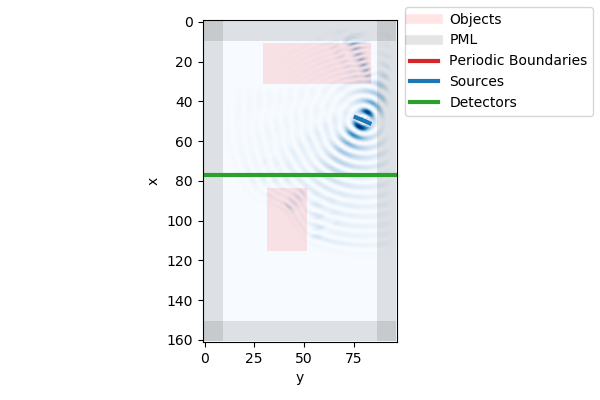
Grid visualization

Let’s visualize the grid. This can be done with the grid.visualize method:

# signature
grid.visualize(
    grid,
    x=None,
    y=None,
    z=None,
    cmap="Blues",
    pbcolor="C3",
    pmlcolor=(0, 0, 0, 0.1),
    objcolor=(1, 0, 0, 0.1),
    srccolor="C0",
    detcolor="C2",
    show=True,
)

This method will by default visualize all objects in the grid, as well as the field intensity at the current time_step at a certain x, y OR z-plane. By setting show=False, one can disable the immediate visualization of the matplotlib image.

grid.visualize(z=0)