04. Performance Profiling

We can profile the performance with a 3D FDTD simulation:

Imports

import matplotlib.pyplot as plt
from line_profiler import LineProfiler

import fdtd
import fdtd.backend as bd

Set Backend

Let’s profile the impact of the backend. These are the possible backends:

• numpy (defaults to float64 arrays)

• torch (defaults to float64 tensors)

• torch.float32

• torch.float64

• torch.cuda (defaults to float64 tensors)

• torch.cuda.float32

• torch.cuda.float64

fdtd.set_backend("numpy")

In general, the numpy backend is preferred for standard CPU calculations with "float64" precision as it is slightly faster than torch backend on CPU. However, a significant performance improvement can be obtained by choosing torch.cuda on large enough grids.

Note that, in FDTD, float64 precision is generally preferred over float32 to ensure numerical stability and prevent numerical dispersion. If this is of no concern to you, you can opt for float32 precision, which especially on a GPU might yield a significant performance boost.

Constants

WAVELENGTH = 1550e-9
SPEED_LIGHT: float = 299_792_458.0  # [m/s] speed of light

Setup Simulation

create FDTD Grid

N = 100

grid = fdtd.Grid(
    (N, N, N),
    grid_spacing=0.05 * WAVELENGTH,
    permittivity=1.0,
    permeability=1.0,
)

add boundaries

# x boundaries
grid[0:10, :, :] = fdtd.PML(name="pml_xlow")
grid[-10:, :, :] = fdtd.PML(name="pml_xhigh")

# y boundaries
grid[:, 0:10, :] = fdtd.PML(name="pml_ylow")
grid[:, -10:, :] = fdtd.PML(name="pml_yhigh")

# z boundaries
grid[:, :, 0:10] = fdtd.PML(name="pml_zlow")
grid[:, :, -10:] = fdtd.PML(name="pml_zhigh")

add sources

grid[10+N//10:10+N//10, :, :] = fdtd.PlaneSource(
    period=WAVELENGTH / SPEED_LIGHT, name="source"
)

[1, 100, 100]

add objects

grid[10+N//5:4*N//5-10, 10+N//5:4*N//5-10, 10+N//5:4*N//5-10] = fdtd.Object(permittivity=2.5, name="center_object")

grid summary

print(grid)

Grid(shape=(100,100,100), grid_spacing=7.75e-08, courant_number=0.57)

sources:
    PlaneSource(period=35, amplitude=1.0, phase_shift=0.0, name='source')
        @ x=[20, ... , 21], y=[0, ... , 100], z=[0, ... , 100]

boundaries:
    PML(name='pml_xlow')
        @ x=0:10, y=:, z=:
    PML(name='pml_xhigh')
        @ x=-10:, y=:, z=:
    PML(name='pml_ylow')
        @ x=:, y=0:10, z=:
    PML(name='pml_yhigh')
        @ x=:, y=-10:, z=:
    PML(name='pml_zlow')
        @ x=:, y=:, z=0:10
    PML(name='pml_zhigh')
        @ x=:, y=:, z=-10:

objects:
    Object(name='center_object')
        @ x=30:70, y=30:70, z=30:70

Setup LineProfiler

create and enable profiler

profiler = LineProfiler()
profiler.add_function(grid.update_E)
profiler.enable()

Run Simulation

run simulation

grid.run(50, progress_bar=True)

100%|██████████| 50/50 [00:12<00:00,  4.03it/s]

Profiler Results

print profiler summary

profiler.print_stats()

Timer unit: 1e-06 s

Total time: 6.15308 s
File: /home/docs/checkouts/readthedocs.org/user_builds/fdtd/checkouts/stable/docs/examples/fdtd/grid.py
Function: update_E at line 291

Line #      Hits         Time  Per Hit   % Time  Line Contents
==============================================================
   291                                               def update_E(self):
   292                                                   """ update the electric field by using the curl of the magnetic field """
   293
   294                                                   # update boundaries: step 1
   295       350       1045.0      3.0      0.0          for boundary in self.boundaries:
   296       300    2281803.0   7606.0     37.1              boundary.update_phi_E()
   297
   298        50    2663606.0  53272.1     43.3          curl = curl_H(self.H)
   299        50     723994.0  14479.9     11.8          self.E += self.courant_number * self.inverse_permittivity * curl
   300
   301                                                   # update objects
   302       100        435.0      4.3      0.0          for obj in self.objects:
   303        50      59449.0   1189.0      1.0              obj.update_E(curl)
   304
   305                                                   # update boundaries: step 2
   306       350        632.0      1.8      0.0          for boundary in self.boundaries:
   307       300     419090.0   1397.0      6.8              boundary.update_E()
   308
   309                                                   # add sources to grid:
   310       100        141.0      1.4      0.0          for src in self.sources:
   311        50       2852.0     57.0      0.0              src.update_E()
   312
   313                                                   # detect electric field
   314        50         36.0      0.7      0.0          for det in self.detectors:
   315                                                       det.detect_E()

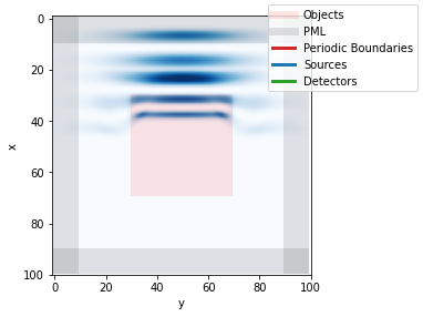
Visualization

plt.figure()
grid.visualize(z=N//2)